hpc futures - part one
Anyone reading my twitter feed will know that I’ve been going to strategy meetings a lot lately. We’ve been talking a lot about the impending problems with computing as new architectures become more complex. By way of organising my thinking about increased resolution, and in some ways, following up on an even older discourse, I’ve spent a bit of time thinking about computing capacity. Hence this.
Currently, European climate computing exploits a range of computing environments. It is common to classify computing environments using a pyramid structure like this:
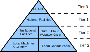
Here we see that Tier0 are the fastest supercomputers available, typically in or close to the top 10 in the world (currently, in Europe, that would mean a PRACE supercomputer, although sometimes ECMWF squeaks into or close to that category, when they have a new computer).
Tier1 computers are typically the fastest computers available nationally for academic use (in the UK that would be Hector). ECMWF is also tier1. Tier2 computers will include institutional supercomputers and the sorts of computers deployed at the Met Office Hadley Centre and DKRZ (although occasionally, when new, they might rank as Tier1).
Large clusters are typically available in institutions too, and often access to these can be achieved via Grid tools. Volunteer grids (access to the personal computers of volunteers via services such as BOINC) are also available. The total amount of computing power available in volunteer grids (measured in FLOPS) exceeds that of the Tier0 supercomputers, but I’ve ranked it as Tier2 here because there are major limitations in what can be done with data flow with such computing - but even so, projects such as climateprediction.net have shown remarkable ability to exploit that environment.
Tier3 computing is what is typically available to a workgroup, which might include local condor pools.
To try and get a grip on trends on what climate computing will be available in in the next decade or so, I’ve been reading this useful SCIDAC review (if you’re at all interested in HPC computing futures, it’s compulsory reading). Following their figure 2, I produced this one:
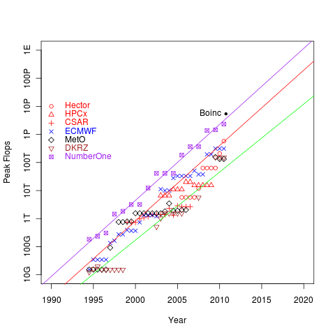
I’ve plotted the theoretical peak FLOPS for major climate computing sites plus ECMWF (not really a climate computer) and the number one computer (in the top500, for comparison) as a function of time. I’ve also plotted the actual throughput of BOINC for June/July 2010. We’ll come back to BOINC. I’ve added three lines: the best fit to the number one computer (purple), the best fit to the leading climate computer (red), and the best fit to the bottom of the climate computing systems (green). Hereafter I’ll imagine the latter are typical of tier1 and tier 2. (I suspect the green line is pretty close to number 500 on the top500 …)
There are some interesting conclusions one can draw:
- HPC follows a nice Moore’s law trajectory and has continued to do so even now that clock speeds are no longer increasing. Of course that’s because of increased parallelisation (of which more later).
- To first order, the average difference between the number one computer, and the best available for climate computing is a difference in power of about 10, and there is a difference in power of about a factor of 10 back to the tier2 computers.
- However, currently it’s important to recognise that the climate share of Tier1 machines is often limited, so in practice, we can think of the horsepower currently available to climate computing (in Europe) as generally being of tier2 class.
- That means, right now, if the money were there, in theory we could get a 100-fold increase in HPC for climate computing by obtaining a tier0 climate computer - however, there is one big gotcha: few (if any) climate codes would scale well on current tier0 architectures … but see below on why that’s not necessarily a problem.
- Even if we had an ECMWF equivalent for climate, it’d be unlikely to exceed the capability of ECMWF, so we could expect to be sitting on tier1 capacity (the same argument applies to climate access to PRACE, 10% of a tier0 will be roughly a tier1 machine).
- It takes roughly three years for tier0 capacity to become available at tier1 and another three to get to tier2.
- BOINC doesn’t actually provide much increase over the capacity of the best available HPC systems (although clearly it’s an important source of computing cycles).
- We can expect the first exascale systems before 2020, and they will be available for tier1 in roughly 2022, and tier2 in 2025-2028 (the line for tier2 seems to be falling away, but I don’t think we should read too much into that, the problem is that the MetO and DKRZ weren’t always in the top500, so the line at the bottom is poorly sampled).
- Similarly, petascale systems will be (in principle) available for climate from next year, but more practically from around 2014-2015.
With those gross generalisations in mind (and hoping the financial situation doesn’t impede capacity provision), let’s return to how increases in computer power can be used by the climate community. Folks have been showing a variant of the following figure (from Tim Palmer at ECMWF) for a long time:
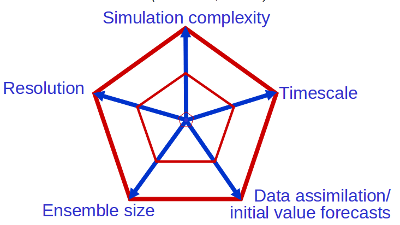
The bottom line is that extra computing can be used in a variety of ways:
- Increased Resolution - horizontally and vertically
- Increased Model Complexity - more processes and sub-models
-
More Ensemble Members
- Better initialisation (data assimilation)
-
Longer duration runs, and
- More Experiments
… and all of them are important to different parts of the spectrum of questions we need to answer, for example:
- Increased resolution and/or complexity will address issues of model uncertainty and applicability to impacts and adaptation
- More ensemble members gives a better sampling of the future and a better handle on uncertainty
- More experiments address all issues, but for example, might allow more scenarios to be explored, and better model validation.
- longer duration runs allow us both to predict further into the future, but also do much longer paleo runs. Paleo runs are an important part of validating our models.
- Better initialisation should allow us to predict the next few decades with less uncertainty.
(For discussions on uncertainty in models, I highly recommend these web pages.)
Not all of these options are equal in our ability to exploit new supercomputing. As hinted above, even now, climate codes can’t necessarily exploit the new computer architectures to either run faster (by using more processors) or go to higher resolution (using more processors), since they don’t necessarily scale well. This has actually been a problem for a while, but it’s been sort of hidden since of late the science drivers have been to more complexity and more ensemble members, and those avenues have tended to better exploit more processors. However, with an increased interest in adaptation and the desirability to do longer runs, comes a necessity to make our models scale. (Really long duration runs at high complexity are going to be a problem, we can’t parallelise in time, yet …)
Of course we can always choose to back-off and loose complexity or resolution to make other kinds of problems doable: for example, really long paleo runs are generally done with lower resolution models with more parameterised physics (but sometimes more complex carbon cycles). Similarly, by staying at lower resolution, climateprediction.net has taken the philosophy that more experiments and more ensemble members can be exploited by using volunteer grids. All of these approaches are valid and useful.
Looking forward however, we do have a problem. If we want to be able to choose which of these avenues to pursue on science grounds rather than computing capability grounds, we need to understand what that computing capability is going to look like, and plan accordingly. More of that anon, when as you might expect, a bit more discussion of data implications will appear.