The Exascale Challenge to the UK - Part Two - Compute
Last time I set up the generic exascale challenge, this time I want to discuss how it is playing out here and now for UK climate modelling. This long-ish post discusses computer hardare and benchmarking of our codes. The next one will discuss the implication for science.
One of the things we have recently been trying to do is size the sort of models we might be able to run on the next generation national HPC platform (whatever that might be) and potentially on the pre-exascale and exascale machines we might see in Europe in the next decade. You might wonder why we’re thinking that far ahead, but the bottom line is that it takes years (up to a decade) to develop a (good) model, and we need to be thinking about what modelling programmes we can do with the models we have now, or will have soon, and what models we need to build/acquire/alter.
We have to do this amongst the usual uncertainty in what computing is available, or might be available. There are a couple of constraints: we know that the current generation of the Unified Model gets no benefit from GPU technology, so we’re really going to be looking at CPU variants, and today that would mean some kind of Intel chip - Broadwell, Skylake etc. In the near future we might hope that someone will build a supercomputer using AMD or ARM chip1.
We don’t have any information about our codes running on AMD silicon yet (if anyone from AMD wants to talk to us about that, please get in touch), but we do have some information about how ARM might play out from the work Simon McIntosh-Smith’s team are doing on the new ISAMBARD platform. He .. talked about this at Supercomputing 2017, and there are two relevant slides to talk about:
Firstly (slide 7 if you look on the link above), he showed some benchmark comparisons of a number of codes on a single socket of Broadwell, Skylake and ThunderX2 arm (with 18, 22 and 32 cores respectively). My reading of these benchmark results are there is a 40-50% improvement between Broadwell and Skylake, and in nearly all cases substantial further improvement in the ThunderX2 results, but not breathtakingly more.
However, more importantly from my perspective are the results using the UM and NEMO on the next slide, where a Broadwell/ThunderX2 comparison shows something like a 40% improvement for the UM (the NEMO results were on a slightly different TX2 platform so I won’t muddy the waters talking about them). The UM speed improvements must be coming from a combination of the extra cores and memory bandwidth on the TX2. Of course there are nearly 2x more cores on the TX2 (32) than the Broadwell (18), so the work done per core is less (which is a good reminder that core-hours are a poor comparative measure).
I’m going to go (not very far) out on a limb and suggest then there is likely about 50% performance advantage between Broadwell nodes and anything we might buy in the near future (less than two or so years) with either Skylake or ThunderX2 nodes.
We have access to a Broadwell system - the NERC NEXCS platform (which actually runs on the Met Office’s Cray XCS-40), so we can establish some benchmarks against which we can utilise that 50% extra speed we might get in the future. We don’t currently have access to a Skylake machine, but we can look at evolution between processors by comparing our results with an Ivy-Bridge machine (ARCHER, a Cray XCS-30).
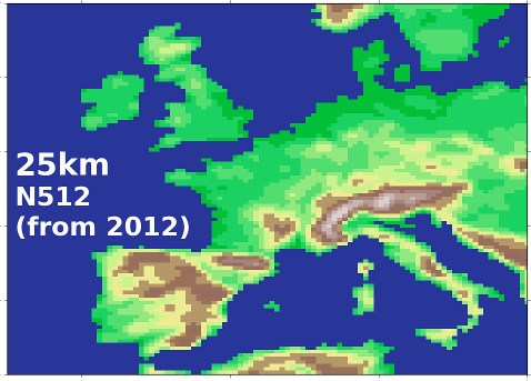
The following data 2 is from an N512 version of the Unified Model. We first started using this resolution around 2012 as part of the UPSCALE project - but despite being five years old, it’s still classed as a high resolution climate model. The N512 grid has different spatial resolution at different latitudes, but we tend to call it a 25km class model. To get a sense of what that means, this is what the European orography looks like at N512:
Ok, so to the data. We have two plots, one where we ran the model without the normal output of variables (for some reason we say “no I/O” when really what we man is no “O”), and one with the normal:
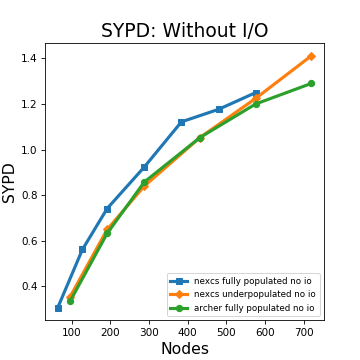
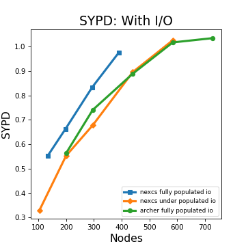
There are three lines on each plot: the results from using all 36 cores on our two-socket Broadwell nodes on NEXCS, from just using 24 cores on NEXCS (so-called “under-populated”) and results from the Ivy Bridge on ARCHER. What we are showing is how many simulated years we can get from one day of computer time as a function of the number of computer nodes we use for the simulation.
There are some quick conclusions we can draw with confidence:
- Core for core we’ve got no benefit from the advances between Ivy-Bridge and Broadwell (!), but
- Clearly node-for-node, we have got a substantial speed up, but it’s nothing like the 50% one might expect from having 50% more cores!
-
At least in this configuration, writing data slows the model down rather a lot.
With slightly lower confidence we can conclude that
- the machines have sufficient interconnect bandwidth, and that maybe the interconnect latency is constraining scaling (Given scaling performance will be function of the code, the interconnect latency, and the inter-connnect bandwidth, and these two machines have the same interconnect latency but differing bandwidth at the largest scale, the fact that they scale the same suggests the constraint is not the bandwidth).
So what? Next time I’ll discuss what this means for advancing our science. I’ve been blogging about this for a long time, since 2005 in fact, so as part of that I’ll be looking at our (my) predictive power.